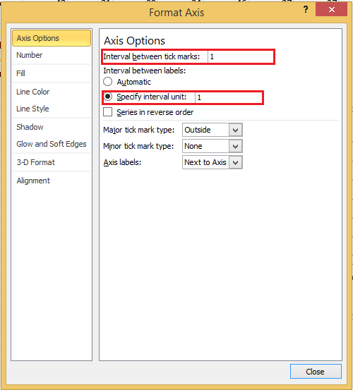
When you insert a chart in Excel, the program might automatically display a chart title or a legend. In cases where Excel omits these labels or they don't adequately explain the chart, turn on axis titles in Excel 2013's Chart Elements menu or the Layout tab in earlier versions of Excel. The top axis options can be adjusted – for example you could change the scale to start 1 Jan 1969 and end 31 Dec 1981 or change the unit settings so there’s not so many labels along the axis. Don’t be afraid to tinker with the chart settings and formatting because Undo is your friend and constant companion.

Editor's note: In the video, Brandon Vigliarolo uses and walks through the steps of building dynamic charts in Excel. The steps are very similar to the following tutorial by Susan Harkins.

If you want to advance beyond your ordinary spreadsheet skills, creating dynamic charts is a good place to begin that journey. The key is to define the chart's source data as a dynamic range. By doing so, the chart will automatically reflect changes and additions to the source data. Fortunately, the process is easy to implement in Excel 2007 and 2010 if you're willing to use the table feature. If not, there's a more complex method.

We'll explore both. SEE: (Tech Pro Research) The table method First, we'll use the table feature, available in Excel 2007 and 2010—you'll be amazed at how simple it is. The first step is to create the table.

To do so, simply select the data range and do the following: • Click the Insert tab. • In the Tables group, click Table. Mac store for windows. • Excel will display the selected range, which you can change.

If the table does not have headers, be sure to uncheck the My Table Has Headers option. • Click OK and Excel will format the data range as a table. Any chart you build on the table will be dynamic. To illustrate, create a quick column chart as follows: • Select the table. • Click the Insert tab. • In the Charts group, choose the first 2-D column chart in the Chart dropdown.

Now, update the chart by adding values for March and watch the chart update automatically. The dynamic formula method You won't always want to turn your data range into a table. Furthermore, this feature isn't available in pre-ribbon versions of Office. When either is the case, there's a more complex formula method. It relies on dynamic ranges that update automatically, similar to the way the table does, but only with a little help from you.

Using our earlier sheet, you'll need five dynamic ranges: one for each series and one for the labels. Instructions for creating the dynamic range for the labels in column A follow. Then, use these instructions to create a dynamic label for columns B through E. To create the dynamic range for column A, do the following: • Click the Formulas tab. • Click the Define Names option in the Defined Names group. • Enter a name for the dynamic range, MonthLabels.