Excel Tips for Mac and PC. Jump to Excel for Mac Jump to Excel for PC. Excel for Mac Basic Excel for Mac. Download Workshop Handout (pdf) Cells, columns, and rows. Raspberry pi 3b downloads. Pivot Tables Tutorial Videos for Mac: Get started Create your pivot table. Refine or re-define your table Use filters and sorting, add a secondary criterion. Learn how to add a secondary axis to your Excel charts on a Mac, PC, or in a Google Doc spreadsheet. Or in a Google Doc spreadsheet. Learn how to add a secondary axis to your Excel charts on a Mac, PC, or in a Google Doc spreadsheet. Check out this tutorial on how to create a pivot table. Originally published Sep 26, 2018 8:13:00 PM.

Pivot tables are excellent for summarizing numbers. At one of my Power Excel seminars recently, someone wanted to show a text field in the Values area of a pivot table. Thanks to the Data Model and the new DAX function CONCATENATEX introduced in 2017, you can build such a pivot table. The attendee said, “I have a data set showing the prior and current status for support tickets. I want to report the text from the Status field in the Values area of a pivot table.” While the Data Model, introduced in Excel 2013, and CONCATENATEX provide a solution, these calculations are only available in Windows versions of Excel.

They won’t work in Excel for Android, Excel for iOS, or Excel for Mac. DAX stands for Data Analysis eXpressions. The DAX formula language is a new set of functions for creating calculated fields in a pivot table. While many of the functions are similar to the functions in regular Excel, there are several powerful additions that allow calculations previously impossible in a pivot table.

In order to use DAX in a pivot table, follow these steps: 1. Select one cell in your data set and press Ctrl+T (or go to Home, Format as Table). By default, the new table will be called Table1. Click on the Table Tools Design tab in the Ribbon and assign the table a name. The table name can’t have spaces. A name such as “TicketData” would work.

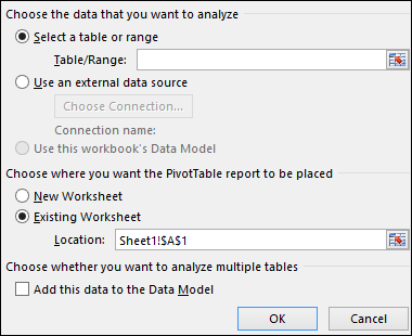
Select one cell in the table. From the Insert Tab, choose Pivot Table. In the Create Pivot Table dialog, choose the box for “Add this data to the Data Model.” 5. A new worksheet will appear with the Pivot Table Fields list. Start to build your pivot table by dragging fields to the Rows and Columns area. When your pivot table is based on the Data Model, there will be a few subtle differences in the Pivot Table Fields list.

First, the words “Active and All” allow you to add more data sets to the pivot table. Second, the name of the table appears at the top of the fields from that table. Right-click the name of the table and choose Add Measure. Note: The word “Measure” is a database professional’s word for Calculated Field.

When the Power Pivot add-in debuted in Excel 2010, the calculated fields were called Measures. Microsoft tried to soften the word in Excel 2013, and the menu choice in Figure 1 appeared as Insert Calculated Field. This was designed to be more familiar for people using Excel. But Excel pivot tables already offer a different feature called Calculated Fields. To avoid confusion, the term changed to “Measure” in Excel 2016. I would have preferred a completely new term, such as “Super Amazing Calculated Field.” 7.

In the Measure dialog, type a measure name such as “StatusResults.” 8. Enter the formula =CONCATENATEX(TicketData,[Status],”, “). Click the Check DAX Formula button to make sure the syntax is correct. You can specify the number format for Measures, which I think is great. For a text result, however, the only valid choice is General, so leave the number format as General. Note: The syntax for CONCATENATEX is (Table Name, Expression, Delimiter).

In the formula in Step 8, TicketData corresponds to the name that you used in Step 2, and [Status] is the name of the field in the source data. To use the AutoComplete feature in the Create Measure dialog, type a left square bracket. The AutoComplete list will show a list of fields from your data set. Click on one name, and press Tab. Click OK to create the new calculated field. The calculation won’t show up in the pivot table automatically. Instead, a new field will appear in the Pivot Table Fields list.